How to get Insights from Spatial Data without SQL

Spatial data analysis celebrates growing user adoption worldwide. There are numerous possibilities of the tools and techniques one can use to get to the desired insights, which are mostly used by the Spatial Data Scientists - a special kind of data scientist who can work with spatial data. But do you really have to be a Spatial Data Scientist to be able to get insights from spatial data? Of course not; it is just a matter of the tools you are using.

For obvious reasons, today, we will talk about how CleverMaps can work for any kind of data scientist, analyst, developer, or enthusiast to get insights from spatial data without special spatial know-how.

SQL: the go-to language for metrics calculation in Spatial Data Analytics

SQL remains the standard language for managing data, but a lack of full training in SQL or understanding of how to use it properly, especially in the spatial context, can prevent you from having a dynamic analytical dashboard with full control at your fingertips… and that's what you need to get to the insights.

Dashboards are composed of metrics. A metric is any collectible, quantifiable measure that enables one to track the performance of an aspect of your product or business over time. Examples of typical metrics in a Location Insights Dashboard:

Sum of all residents
Sum of all customers
Average purchase value per customer
Number of residents per branch
Turnover per resident

To fully understand this point, let's take a closer look at metrics, their usage, and their link to SQL. The main disadvantage of SQL is that it does not have any representation for aggregated numbers for metrics. That means you must calculate them from the bottom up, and SQL requests for the calculation of the given metric must be sent manually in most location analytics tools.

Logical data model and predefined metrics = no manual SQL requests

CleverMaps, the location insights platform, is based on the logical data model and a query engine that creates the SQL requests automatically. For some, this may be the elegant way how to get insights from location data because it can save time, be more efficient and does not require any special spatial data expert.

All the metrics are predefined, so the platform allows you to perform direct calculations on the frontend, such as changes in aggregations, granularity, filters and visualisations. This allows you to slice and dice the metric and evaluate the hypotheses. To do this manually in SQL, it would mean writing dozens of SQL queries as each query gathers data for one particular use-case.

This article will show below how it works in our CleverMaps Studio. CleverMaps is an API-first platform, so another way how to use the technology to your benefit is to build your own application on top of the CleverMps technology.

Building Queries in CleverMaps

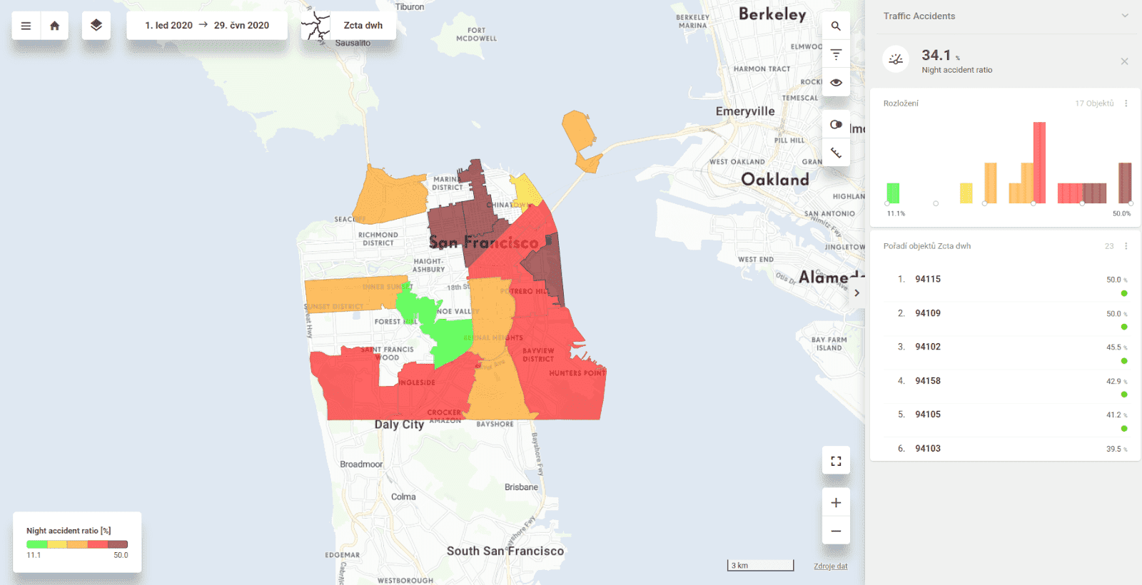
The figures below show one of the views from a project that analyses traffic accidents in San Francisco between 2016 and 2020.

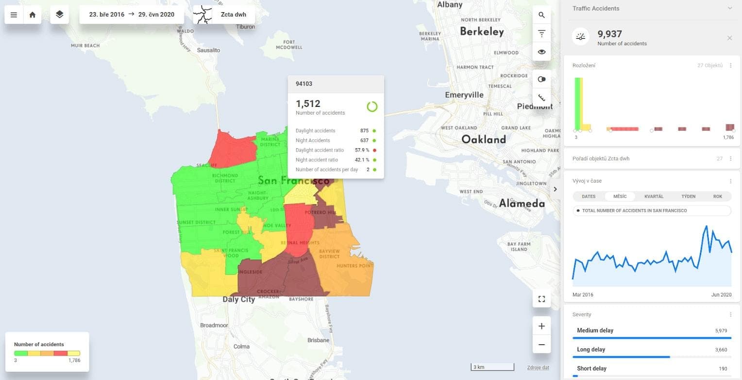
All of the information is computed from one table. To compute all the figures above, you must define SQL queries for traffic accident metrics (count(sf_accidents.id)) in the following variations:

without any aggregation (top right number on the dashboard)
aggregate by severity, by the day, by the hour, by the side of the accident and all other categories that are included in the table (total of 17 different categories)
break down by five or more buckets - to get the histogram view (distribution of traffic accidents based on the area)
aggregate by city zip codes and order by city zip codes to get the areas ranked in order from the highest to lowest

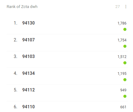
This figure above shows how CleverMaps automatically ranks the zip codes in San Francisco County (left column) and counts the number of accidents for each zip code (right column):

aggregate by Day/Week/Month/Year to show the time series block
compute the average number of accidents per day as well as aggregation for each zip code and other granularities (in the tooltip)
aggregate accidents by night and day
compute ratios for night and day accidents

Once you define these SQL statements, you get a static view showing the screenshot above. Sounds like a lot of work, right? Well, this is where the power of the CleverMaps platform really helps. Just imagine all the queries that you would need to script for getting this data analysis:

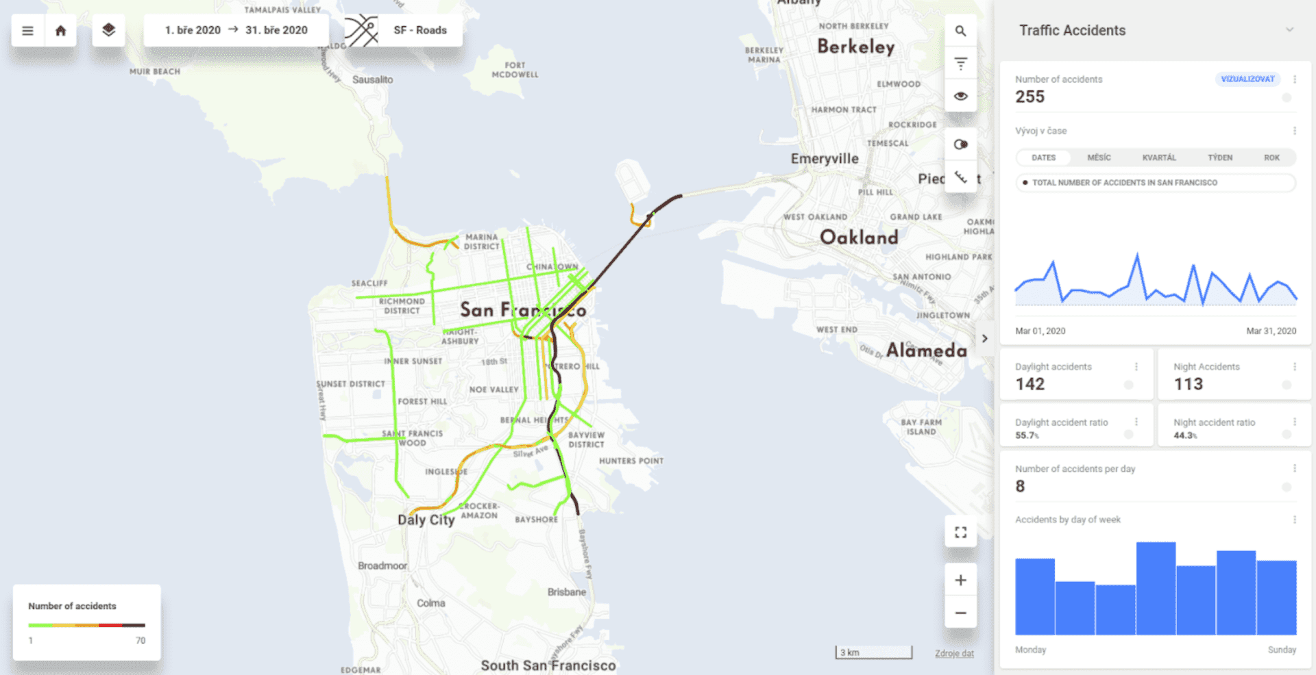
change default granularity to grids or roads
filter data for July 2020 and group them by roads and also roads segments
show all the values above for any random place on the map (that is what the heat map allows you to do)
detect the most dangerous roads in 2020 (filter average number of accidents per day > 2 together with the year filter)

Joining tables with zero effort

We can also switch to another view of the project. This one joins two tables (or more if you need them). Imagine what you would need to perform in SQL to get what CleverMaps can compute on the fly simply by defining a single metric? After that, the UI interacts with the user, and based on filtering, all metrics are automatically recounted, and after one click, the results are visualized in the map.

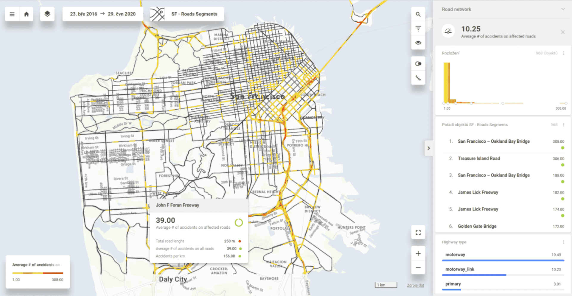
The picture above demonstrates how two tables can join together with zero effort. The first dataset is the one with traffic accidents, and the second one carries the roads and all the necessary information - the names and the types of roads and their length.

As a result, we can filter the most dangerous roads or road segments with the highest average number of accidents on each type of highway per any time window.

Now you can probably imagine that handling all these scenarios could be tricky when using traditional SQL.

To simplify the project building process, we use a logical data model like this:

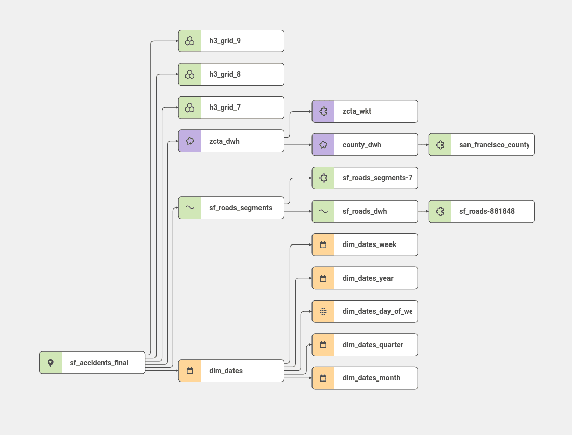
All datasets are logically joined together. In this case, all datasets except the sf_accident and the roads related dataset had been imported into the project since these dimensions are already pre-set and joined together, specifically the uber grid, dates and polygons.

Let's take it to practice

The data model describes datasets and their relations with each other in the project. On top of the model and selected dataset, we define a logical metric. For example, in the case of traffic accidents, it is a simple count over the id of each accident like this: COUNT(sf_accidents.id).

The next step is to define an indicator, which establishes the formatting and labeling of the metric. The indicator is then directly placed on the dashboard. After that, you create an indicator drill that helps you define all the categories in which you would usually group the table in SQL.

And that's it! The CleverMaps application can show all the available granularities, compute all the blocks, and show all tooltips on the map based on the initial metric. This process is seamless, and anytime you add a new dimension of granularity (eg. Grid) it will be recalculated instantly. Likewise, anytime you add a new global filter, it will overwrite all applicable metrics.

Definition of metric representing the calculation of the night ratio for the year 2020:

           {
"name": "night_ratio_metric",
"type": "metric",
"content": {
"type": "function_divide",
"content": [
   {
"type": "function_count",
"content": [
{
  "type": "property",
   "value": "sf_accidents_final.id_accident"
}
  ],
"options": {
"filterBy": [
{
"property": "sf_accidents_final.sunrise_sunset",
"value": "Night",
                             "operator": "eq"
                         }
                     ]
                 }
             },
             {
                 "type": "function_count",
                 "content": [
                     {
                         "type": "property",
                         "value": "sf_accidents_final.id_accident"
                     }
                 ]
        }
]
     }
}

SQL script representing the calculation of the night ratio metric for the year 2020:

select
"zcta_code",
"x_min",
"x_max",
"y_min",
"y_max",
"night_ratio_metric",
count(*) over () as "total_rows_count"
from (
with recursive
   "night_ratio_metric_1" as (
   select
   "zcta_dwh_1"."zcta_code" as "zcta_code",
   count("sf_accidents_final_11"."id_accident") as "night_ratio_metric_1"
   from "sf_accidents_final_11"
   join "zcta_dwh_1"
   on "sf_accidents_final_11"."cm_zipcode" = "zcta_dwh_1"."zcta_code"
   where (
   "sf_accidents_final_11"."sunrise_sunset" = 'Night'
   and "sf_accidents_final_11"."date" >= '2020-01-01'
   and "sf_accidents_final_11"."date" <= '2020-06-29'
   )
   group by 1
   order by "zcta_code" asc
   ),
   "night_ratio_metric_2" as (
   select
   "zcta_dwh_1"."zcta_code" as "zcta_code",
   count("sf_accidents_final_11"."id_accident") as "night_ratio_metric_2"
   from "sf_accidents_final_11"
   join "zcta_dwh_1"
   on "sf_accidents_final_11"."cm_zipcode" = "zcta_dwh_1"."zcta_code"
   where (
   "sf_accidents_final_11"."date" >= '2020-01-01'
   and "sf_accidents_final_11"."date" <= '2020-06-29'
   )
   group by 1
   order by "zcta_code" asc
   ),
   "at_zcta_dwh" as (
   select
   "zcta_dwh_1"."zcta_code" as "zcta_code",
   "zcta_dwh_1"."x_min" as "x_min",
   "zcta_dwh_1"."x_max" as "x_max",
   "zcta_dwh_1"."y_min" as "y_min",
   "zcta_dwh_1"."y_max" as "y_max"
   from "zcta_dwh_1"
   )
select
   coalesce(
   "night_ratio_metric_1"."zcta_code",
   "night_ratio_metric_2"."zcta_code"
   ) as "zcta_code",
   coalesce("at_zcta_dwh"."x_min") as "x_min",
   coalesce("at_zcta_dwh"."x_max") as "x_max",
   coalesce("at_zcta_dwh"."y_min") as "y_min",
   coalesce("at_zcta_dwh"."y_max") as "y_max",
   round((cast("night_ratio_metric_1" as numeric) / nullif("night_ratio_metric_2", 0.0))::numeric, 3) as "night_ratio_metric"
from "night_ratio_metric_1"
   full outer join "night_ratio_metric_2"
   on "night_ratio_metric_1"."zcta_code" = "night_ratio_metric_2"."zcta_code"
   left outer join "at_zcta_dwh"
   on coalesce(
   "night_ratio_metric_1"."zcta_code",
   "night_ratio_metric_2"."zcta_code"
   ) = "at_zcta_dwh"."zcta_code"
group by
   1,
   2,
   3,
   4,
   5,
   "night_ratio_metric_1",
   "night_ratio_metric_2"
order by
   1 asc,
   2 asc,
   3 asc,
   4 asc,
   5 asc,
   "night_ratio_metric_1" asc,
   "night_ratio_metric_2" asc

) as "inner"
where (
"y_max" > 37.66105827154423
and "y_min" < 37.886841225353955
and "x_max" > -122.87075042724611
and "x_min" < -121.99184417724611
)
limit 20000
offset 0

Leverage the technology in your data stack

This article showed you how the CleverMaps Studio interacts with CleverMaps logical data model and spatial query engine. In case you already built your mapping solution or the CleverMaps Studio is not quite what you are looking for, you can leverage only the technology on the back end and integrate it to your solution with our REST API.

Want to try it out? You can build your project with our templates.

If you are interested in finding out more about the possibilities of the CleverMaps platform, you are very welcome to schedule a demo with us!

I want to know about next new article

Leave us your e-mail to receive news about Location Intelligence and the CleverMaps platform itself.

By checking this box, I agree to receive a business communication from CleverMaps and to process my personal data in accordance with the CleverMaps Privacy Policy (see the link in the website footer). I understand that I can withdraw my consent at any time.